Week 9 - Natural Language

IAT 461 / 882 · Data Science for Human-Centered Systems · Summer 2026 · Alireza Karduni

The Problem

Moderating Twitch Chat

• Twitch chat moves fast — thousands of messages per minute on large streams
• Moderators can’t read everything in real time
• We want a model that flags abusive messages automatically

Is This Message Abusive?

viewer1: trash uninstall noob

viewer2: well played gg

viewer3: you're actually trash at this game

viewer4: that boss fight will kill me 😭

Which ones are abusive? It’s not always obvious.

Why Is This Hard?

• The same word shows up in both contexts — “kill” in a game complaint vs. a threat
• Sarcasm and tone don’t show up in text alone
• Slang and spelling evolve constantly to evade filters
• Millions of messages — moderation has to be automatic and fast

Reframing the Problem

• Input: a chat message (text)
• Output: a label — Abusive or Clean
• This is a classification problem

But models compute with numbers, not sentences. First, we need to turn text into numbers.

From Text to Numbers

Models Need Numbers

• A model can’t read “trash uninstall noob” the way we do
• Every model — Naive Bayes included — needs a numeric representation of text
• Getting there takes two steps: tokenize, then count

Tokenization

• Tokenization = breaking raw text into smaller units, usually words
• Sounds simple — but there are choices to make along the way

Tokenization, Step by Step

flowchart LR
  A["'Trash, uninstall!!'"] --> B["lowercase<br/>'trash, uninstall!!'"]
  B --> C["remove punctuation<br/>'trash uninstall'"]
  C --> D["split on spaces<br/>['trash', 'uninstall']"]

Choices in Tokenization

• Lowercase everything? (Trash vs trash)
• Strip punctuation? (gg!!! vs gg)
• Remove common words like “the”, “is”, “you”?

We’ll come back to that last one — for abuse detection, “you” might actually matter.

Our Toy Dataset

#	Message	Class
1	trash uninstall noob game	Abusive
2	idiot trash chat	Abusive
3	well played gg chat	Clean
4	nice play well game	Clean

Small on purpose — small enough to calculate by hand.

Building a Vocabulary

Every unique token across all four messages:

chat, game, gg, idiot, noob, nice, play, played, trash, uninstall, well

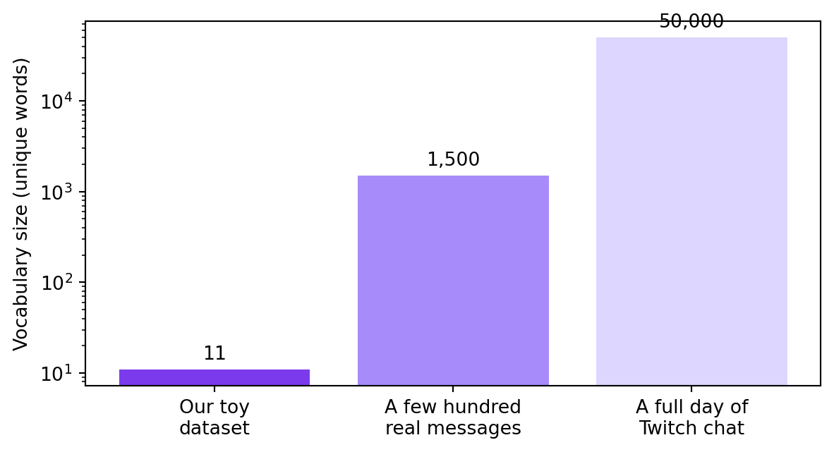
11 words. This is our vocabulary.

Count Vectors

Each message becomes a row of word counts:

Message	chat	game	gg	idiot	noob	nice	play	played	trash	uninstall	well
1 (Abusive)	0	1	0	0	1	0	0	0	1	1	0
2 (Abusive)	1	0	0	1	0	0	0	0	1	0	0
3 (Clean)	1	0	1	0	0	0	0	1	0	0	1
4 (Clean)	0	1	0	0	0	1	1	0	0	0	1

This is bag-of-words: word order is thrown away, only counts remain.

What We Have Now

• Every message is now a vector of numbers
• We can compare, count, and calculate with these vectors
• Notice: trash appears only in Abusive rows, well only in Clean rows — that’s a signal
• chat and game show up in both Abusive and Clean rows — we’ll see what that does to the math next

Bayes, Revisited

Quick Recall

• We met Bayes’ Theorem earlier this term
• One more pass — this time aimed straight at classification

Bayes’ Theorem

\[P(A \mid B) = \frac{P(B \mid A)\, P(A)}{P(B)}\]

Four pieces. Let’s name each one.

Bayes’ Theorem, in Words

\[P(A \mid B) = \frac{P(B \mid A)\, P(A)}{P(B)}\]

• \(P(A \mid B)\) — posterior: updated belief about \(A\), after seeing \(B\)
• \(P(B \mid A)\) — likelihood: how likely \(B\) is, if \(A\) is true
• \(P(A)\) — prior: belief about \(A\) before seeing any evidence
• \(P(B)\) — evidence: how likely \(B\) is, overall

Swapping in Our Problem

\[P(\text{class} \mid \text{message}) = \frac{P(\text{message} \mid \text{class})\, P(\text{class})}{P(\text{message})}\]

• Posterior — probability the message is Abusive, given the words it contains
• Likelihood — how likely these exact words are, if the message really is Abusive
• Prior — how common Abusive messages are overall
• Evidence — how common this exact message is, regardless of class

Where Does the Prior Come From?

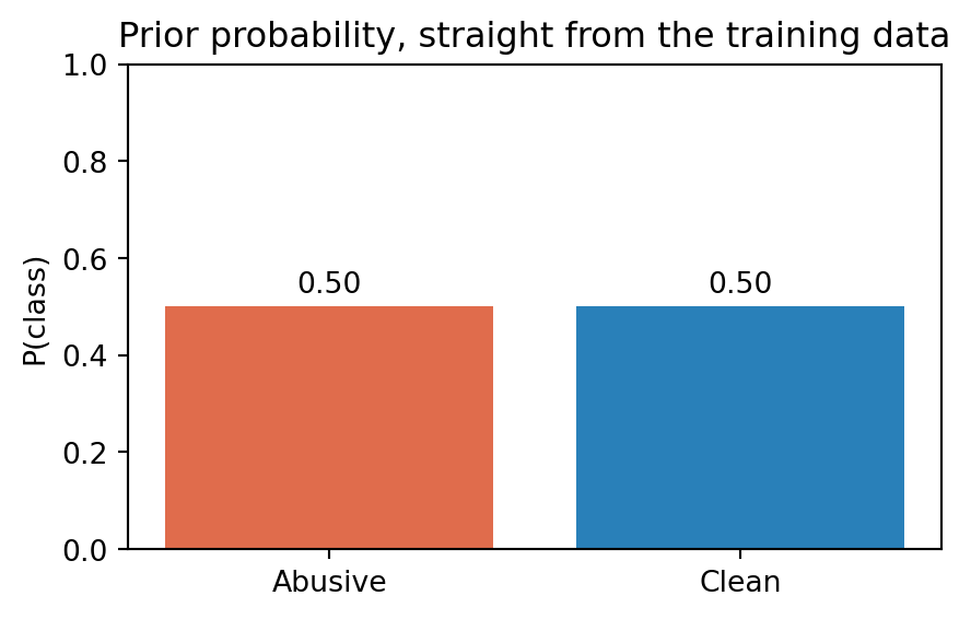
2 Abusive + 2 Clean messages → P(Abusive) = 0.5, P(Clean) = 0.5. No fancy math — just counting.

We Can Drop the Denominator

• \(P(\text{message})\) is the same number no matter which class we’re testing
• To decide between Abusive and Clean, we just need to know which numerator is bigger

\[P(\text{class} \mid \text{message}) \;\propto\; P(\text{message} \mid \text{class}) \, P(\text{class})\]

The Real Challenge: \(P(\text{message} \mid \text{class})\)

• A message is one specific combination of words
• To compute this directly, we’d need to have seen that exact combination many times during training
• We almost never have enough data for that — most word combinations are rare or brand new

Preview: The Naive Assumption

• Naive Bayes assumes each word’s probability is independent of the others, given the class
• That turns one hard combination into a product of easy pieces

\[P(\text{message} \mid \text{class}) \;\approx\; \prod_{i} P(\text{word}_i \mid \text{class})\]

Next: let’s calculate this by hand on our toy dataset.

Naive Bayes: A Worked Example

Setting Up

• Test message: “trash game”
• We compare P(Abusive | message) vs. P(Clean | message)
• Whichever is bigger wins

Step 1 — Priors

• P(Abusive) = 0.5
• P(Clean) = 0.5
• (2 messages in each class, out of 4 total)

Step 2 — Word Counts per Class

Class	chat	game	gg	idiot	noob	nice	play	played	trash	uninstall	well	Total
Abusive	1	1	0	1	1	0	0	0	2	1	0	7
Clean	1	1	1	0	0	1	1	1	0	0	2	8

Vocabulary size: 11 words. Watch trash and game — that’s our test message.

Step 3 — The Likelihood Formula

\[P(\text{word} \mid \text{class}) = \frac{\text{count(word, class)}}{\text{total words in class}}\]

Just a proportion — how often this word shows up, within this class.

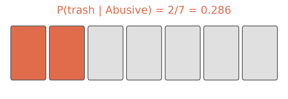
Visualizing P(trash | Abusive)

2 of the 7 words in Abusive messages are “trash.”

Visualizing P(game | Abusive)

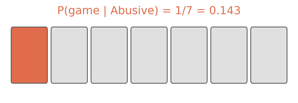
Only 1 of the 7 — “game” shows up, but it’s not a strong Abusive signal on its own.

Visualizing P(trash | Clean)

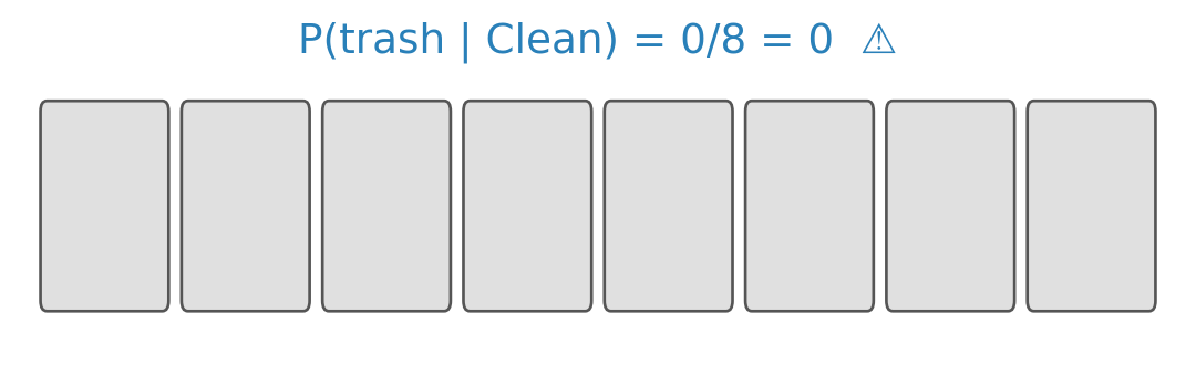
Not one square is colored — “trash” never appears in a Clean message.

Visualizing P(game | Clean)

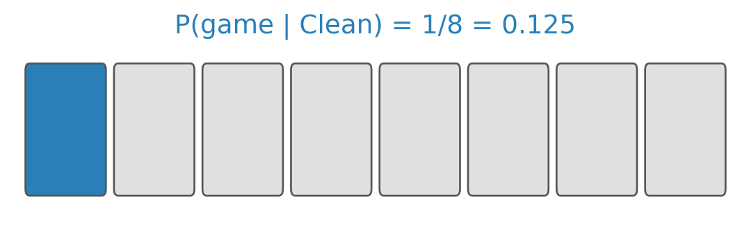
1 of 8 — about the same odds as in Abusive. This word isn’t telling us much.

That’s a Problem

• One missing word shouldn’t be an absolute veto
• P(trash | Clean) = 0 → the entire message probability collapses to zero, no matter what else is in it
• Real vocabularies have thousands of words — most won’t appear in every class

Step 5 — Laplace (Add-1) Smoothing

\[P(\text{word} \mid \text{class}) = \frac{\text{count(word, class)} + 1}{\text{total words in class} + |V|}\]

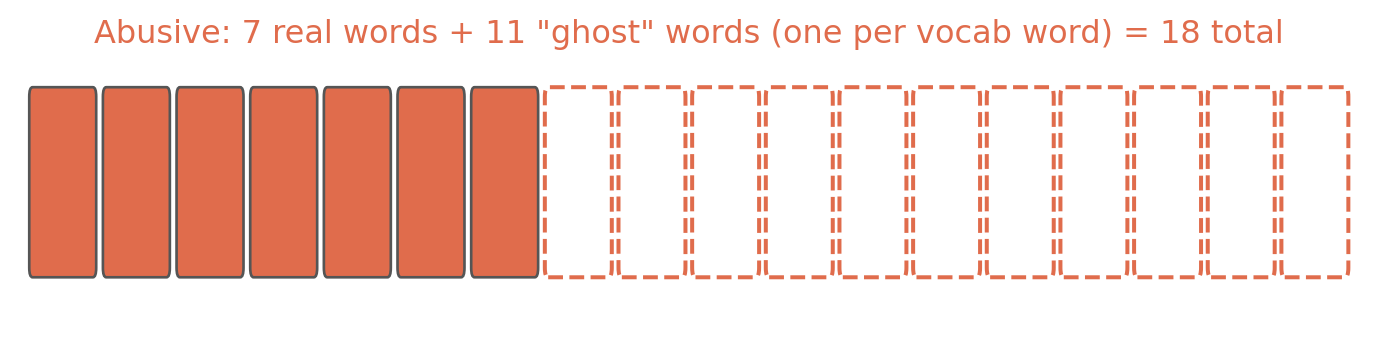
• Pretend every word in the vocabulary appeared one extra time, in every class
• Guarantees no probability is ever exactly zero
• \(|V|\) = vocabulary size = 11

Smoothing, Visualized

Same idea applies to Clean: 8 real + 11 ghost = 19 total.

Step 6 — Recalculated, Smoothed

Class	P(trash | class)	P(game | class)
Abusive	(2+1)/(7+11) = 0.167	(1+1)/(7+11) = 0.111
Clean	(0+1)/(8+11) = 0.053	(1+1)/(8+11) = 0.105

“trash” is no longer a hard zero — just a small number.

Step 7a — Multiplying Word Probabilities

• Naive Bayes multiplies each word’s probability together, per class

\[P(\text{message} \mid \text{class}) = P(\text{word}_A \mid \text{class}) \times P(\text{word}_B \mid \text{class}) \times \dots\]

For “trash game,” each class has exactly 2 words to multiply:

\[P(\text{message} \mid \text{class}) = P(\text{trash} \mid \text{class}) \times P(\text{game} \mid \text{class})\]

Step 7b — Substituting the Numbers

• P(message | Abusive) = 0.167 × 0.111 = 0.0185
• P(message | Clean) = 0.053 × 0.105 = 0.0055

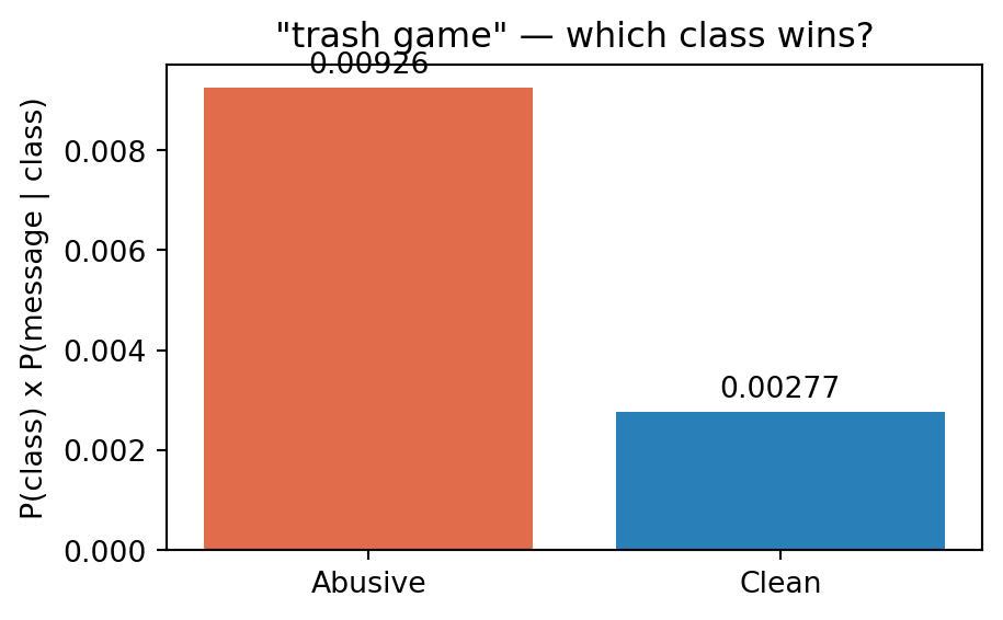
Step 8 — Bring Back the Prior

Class	Prior	× Likelihood	= Posterior (unnormalized)
Abusive	0.5	0.0185	0.00926
Clean	0.5	0.0055	0.00277

Step 9 — Decide

\(0.00926 > 0.00277\) → classify “trash game” as Abusive

Step 10 — What Actually Drove This?

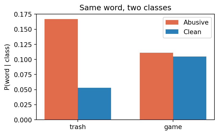
• trash: big gap between classes → strong signal, does the real work
• game: nearly the same height in both → barely moves the decision

Words that show up equally in every class carry little information — the model figures this out from data, without being told which words matter.

Bigrams & N-grams

Recap: The Problem

• Unigrams (single words) throw away order completely
• “not toxic, very kind” and “very toxic, not kind” produced identical count vectors
• We need a “word” that captures a little bit of order

What Is an N-gram?

• Instead of tokenizing into single words, tokenize into sequences of N consecutive words
• \(N=1\) → unigram (what we’ve done so far)
• \(N=2\) → bigram
• \(N=3\) → trigram

From Words to Bigrams

flowchart LR
  A["tokens<br/>[not, toxic, very, kind]"] --> B["slide a window of 2<br/>across the tokens"]
  B --> C["bigrams<br/>[(not,toxic), (toxic,very), (very,kind)]"]

Bigrams of Our Two Messages

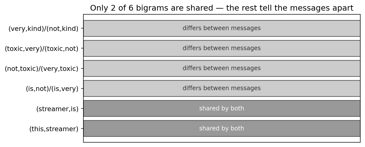
"this streamer is not toxic, very kind"

(this,streamer) → (streamer,is) → (is,not) → (not,toxic) → (toxic,very) → (very,kind)

"this streamer is very toxic, not kind"

(this,streamer) → (streamer,is) → (is,very) → (very,toxic) → (toxic,not) → (not,kind)

Same starting words, but the sequences split apart right where the meaning flips.

Now the Vectors Differ

Naive Bayes now has something to actually distinguish these two messages by.

The Cost: Vocabulary Growth

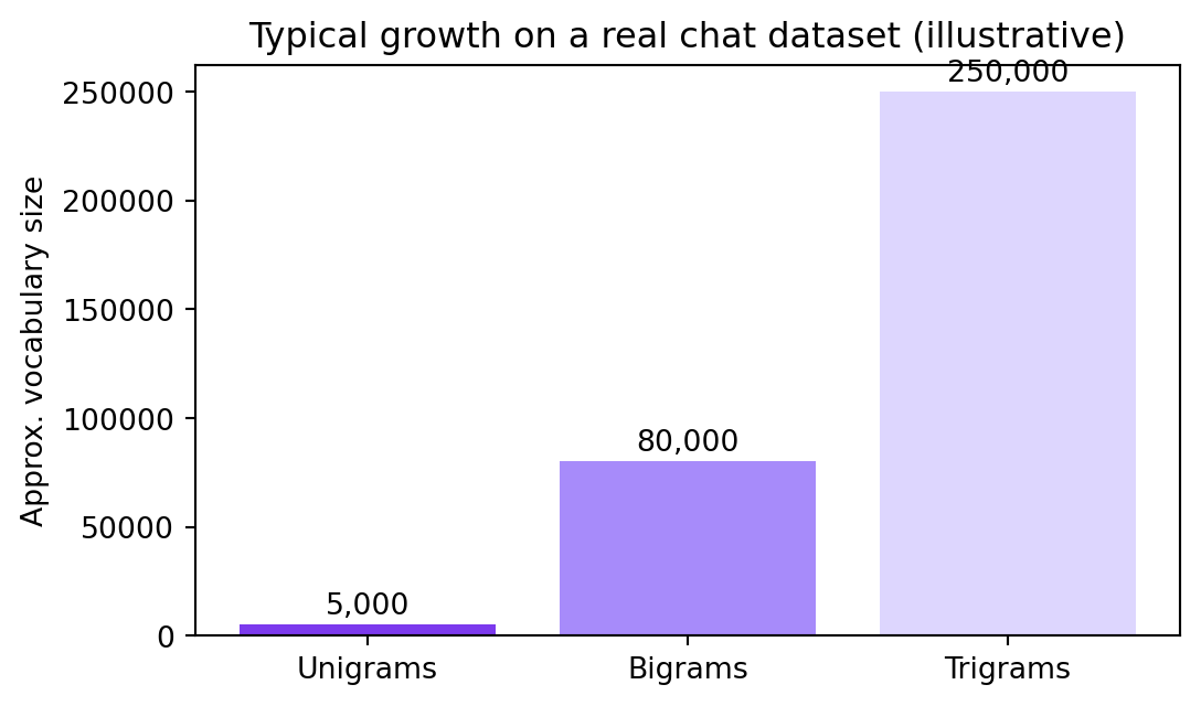
• More context per token = more possible combinations
• Vocabulary grows fast, count vectors get sparser (more zeros)
• Trade-off: better at catching order, harder to get enough examples of every combination

A Bonus: Character N-grams

• N-grams don’t have to be built from words — they can be built from characters
• Useful for catching obfuscated abuse: “idiot” vs. “idi0t”

Character Trigrams, Side by Side

"idiot" → idi   dio   iot

"idi0t" → idi   di0   i0t

Word-level tokenization sees “idiot” and “idi0t” as completely different, unrelated tokens — zero overlap.

Character trigrams still share “idi” — some signal survives the obfuscation.

Choosing a Tokenization Strategy

• Unigrams — simple, fast, but blind to word order
• Bigrams / trigrams — capture some order and phrasing, at the cost of sparsity
• Character n-grams — robust to misspellings and obfuscation, useful specifically for abuse/spam detection
• All of these still plug into the same Naive Bayes math — only how we build the count vector changes

TF-IDF

Recap: What Raw Counts Miss

• Count vectors treat every word the same way — just “how many times did it appear”
• A word that shows up in almost every message isn’t very distinctive, even if its count is high
• We want a score that rewards words that are frequent here, but rare elsewhere

Term Frequency (TF) — A Quick Recap

\[TF(\text{word}, \text{doc}) = \frac{\text{count(word, doc)}}{\text{total words in doc}}\]

This is the same calculation we already did for Naive Bayes likelihoods — just applied per-document here instead of per-class.

The Missing Piece: Document Frequency

• Document Frequency (DF) — in how many documents does this word appear at all?
• Not “how many times” — just “in how many messages, yes or no”

Document Frequency, Our Toy Corpus

Word	Appears in docs	DF
chat	2, 3	2
idiot	2	1
well	3, 4	2

Only 4 documents total in our toy corpus — so DF can only be 1, 2, 3, or 4.

Inverse Document Frequency (IDF)

\[IDF(\text{word}) = \log \left( \frac{N}{DF(\text{word})} \right)\]

• \(N\) = total number of documents
• Rare across the corpus → high IDF
• Common everywhere → low IDF (a word in every doc gets \(IDF = \log(1) = 0\))

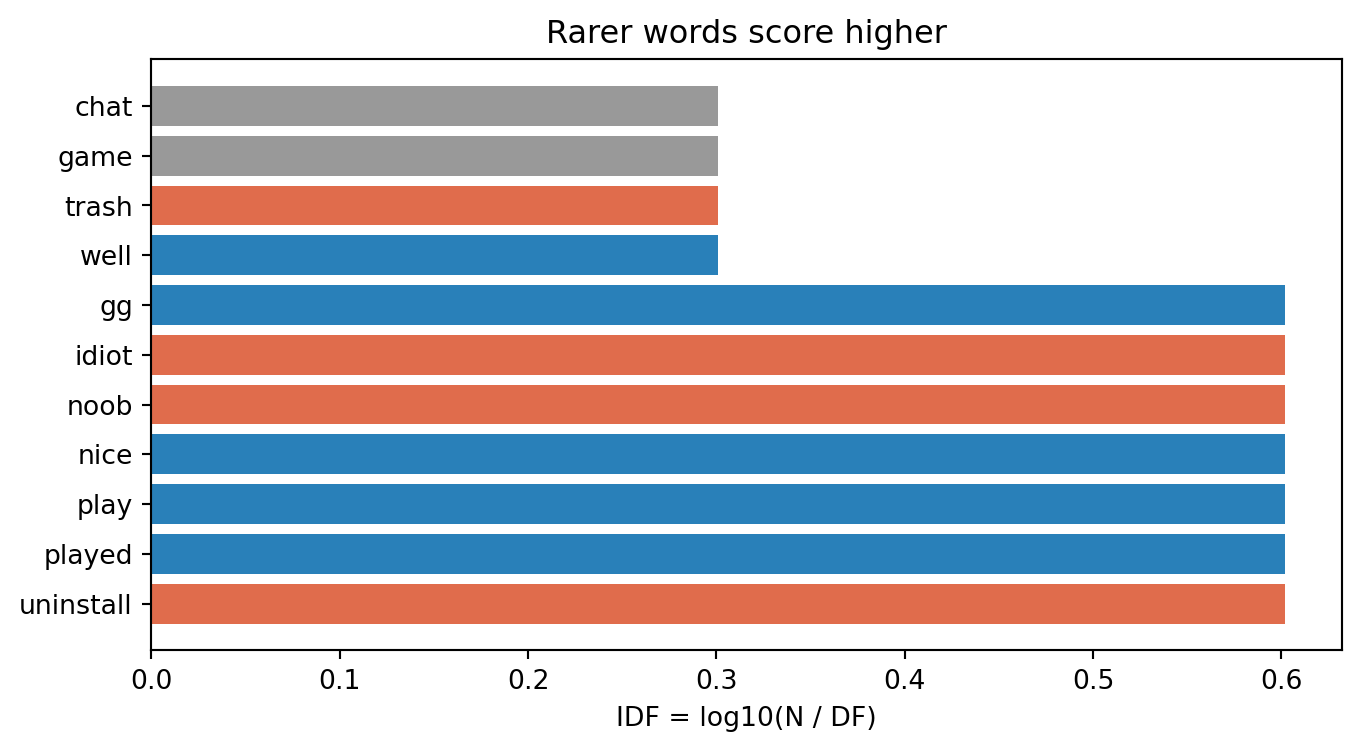
IDF Across Our Vocabulary

Gray = shared by both classes · Red = Abusive-only · Blue = Clean-only

Wait — IDF Doesn’t Know About Classes

• Look at trash and well — both score the same IDF as chat and game
• IDF only counts how many documents a word appears in — it has no idea which class those documents belong to
• A word can be a perfect class signal and still get an unremarkable IDF score

IDF measures rareness, not classification usefulness — those are related, but not the same thing.

TF-IDF: Putting Them Together

\[ \begin{aligned} TF\text{-}IDF(\text{word}, \text{doc}) &= TF(\text{word}, \text{doc}) \\ &\times IDF(\text{word}) \end{aligned} \]

High score = frequent in this message, and rare across the corpus. That’s what makes a word distinctive.

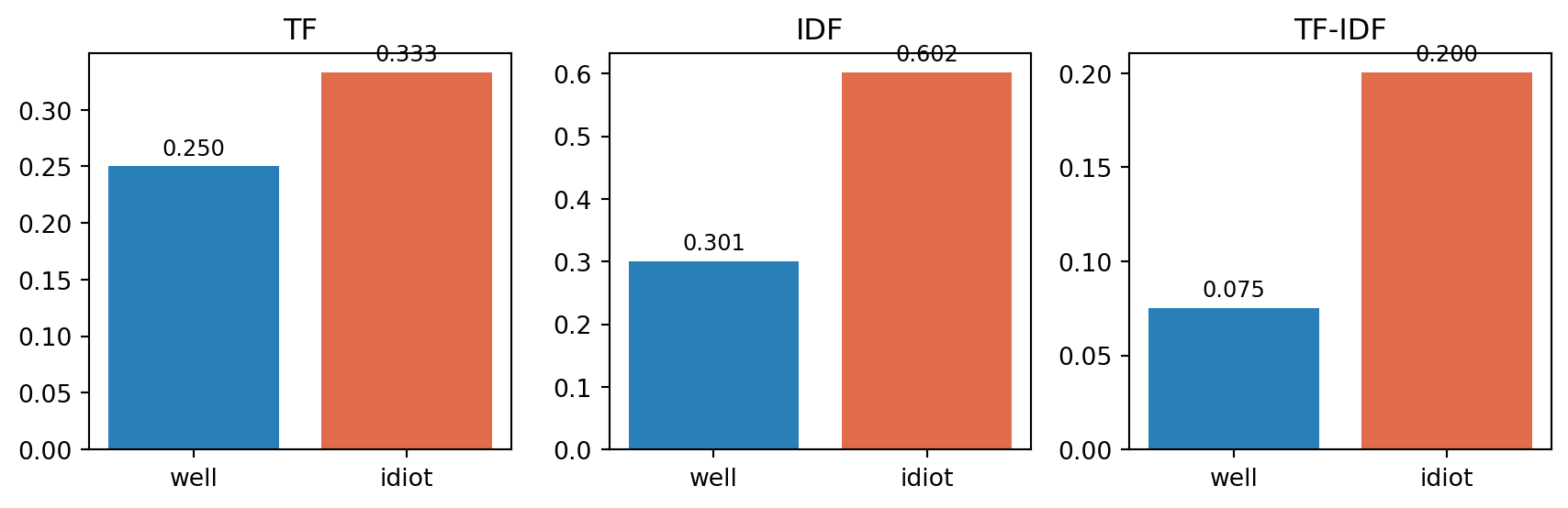
Worked Example: “well” vs. “idiot”

• “well” in doc 3 (“well played gg chat”, 4 words): \(TF = 1/4 = 0.25\), \(IDF = \log_{10}(4/2) = 0.301\)
• “idiot” in doc 2 (“idiot trash chat”, 3 words): \(TF = 1/3 = 0.333\), \(IDF = \log_{10}(4/1) = 0.602\)

The Payoff

Both words appear once in their message — same TF story almost. But “idiot” is rarer across the corpus, so it ends up with the higher TF-IDF score.

Count Vectors vs. TF-IDF Vectors

• Count vector: “how many times does each word appear in this message?”
• TF-IDF vector: “how much does each word actually tell us about this message?”
• Naive Bayes can be built on either — count vectors are the classic version, TF-IDF weighting is a common refinement

Count vectors tell you what’s there. TF-IDF tells you what’s distinctive.

Naive Bayes in Reality

Real Twitch Chat Isn’t 4 Tiny Messages

viewer_882: bro literally uninstall the game already you absolute waste of a human being trash player

gamer_lisa: that was such a clean play omg well done let's gooo nice combo at the end there

tox1c_kappa: everyone in this lobby is actual garbage lmao noob team carried by nobody

Real messages, real vocabulary — nowhere near 11 words.

The Vector Explodes

Each message is still just one row — but now it’s a row with 50,000 columns.

One Message, Mostly Zeros

That’s just 300 columns shown. A real vector might be 50,000 columns wide — almost entirely zero.

What This Means in Practice

• Vectors this sparse are stored as sparse matrices — only the non-zero positions are kept, not 50,000 zeros per message
• Multiplying hundreds of small probabilities together underflows to zero — real implementations sum log-probabilities instead of multiplying raw ones
• The math is exactly what we did by hand — just done at scale, in log-space, with sparse storage

Beyond Naive Bayes: Decision Trees

A Different Kind of Model

• Naive Bayes: probabilistic — multiplies word probabilities together
• Decision Tree: a series of yes/no questions about the message
• No independence assumption at all — a genuinely different paradigm

Starting Point: Six Messages

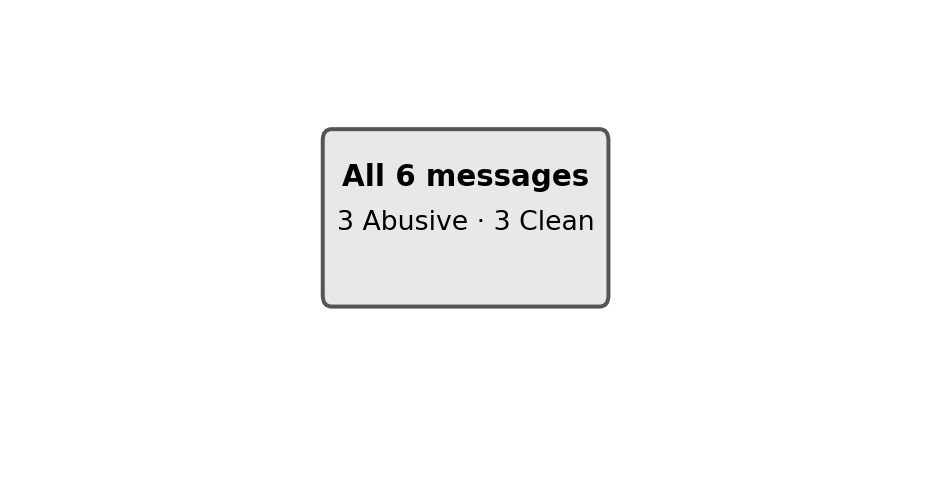
This time, two messages break the pattern: an Abusive one contains “well,” and a Clean one doesn’t.

First Split: “Contains ‘well’?”

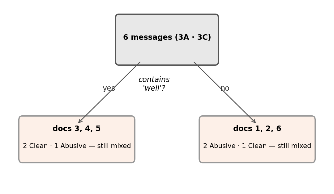
Not a perfect split this time — both sides still contain a mix of classes. The tree needs to go one level deeper.

Left Branch: “Contains ‘trash’?”

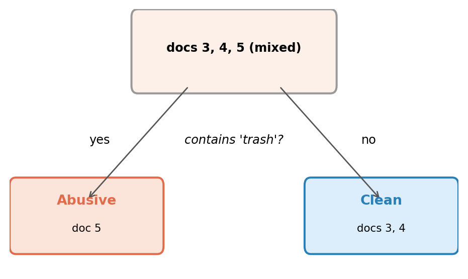
“well trash noob” gives itself away on the second question — pure leaves now.

Right Branch: “Contains ‘nice’?”

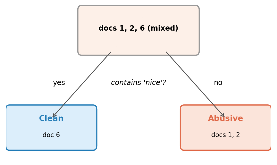
Same idea on the other branch — one more question, and it’s pure too.

The Full Tree

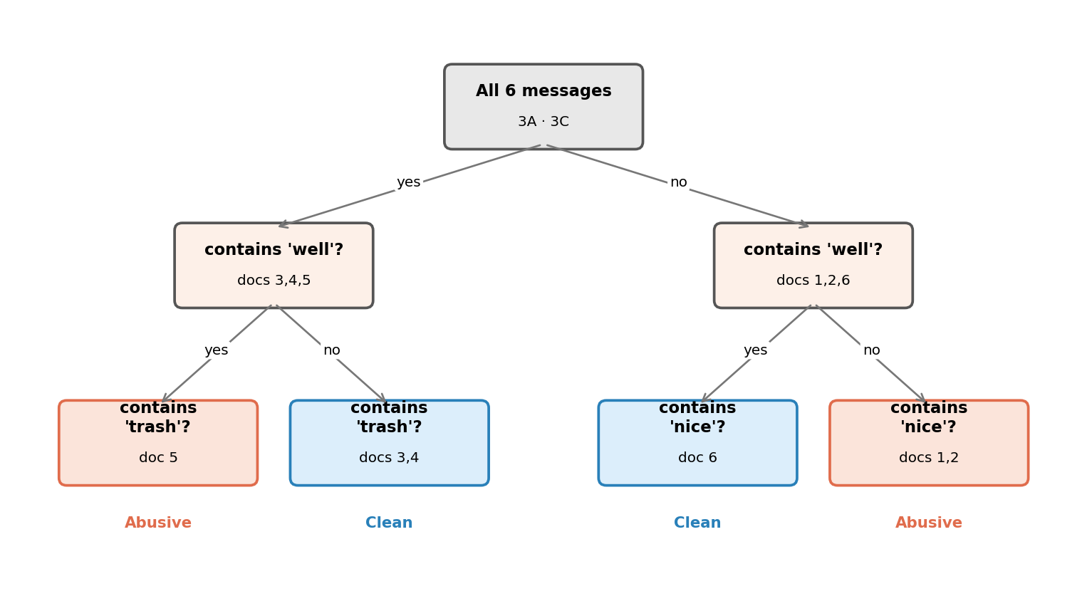
Two levels of questions, four pure leaves. Every leaf now contains only one class.

Worth Noticing

• One of those leaves — “contains trash → Abusive” — has exactly one message in it
• That’s a warning sign, not a triumph: the tree has carved out a rule custom-fit to a single example
• On new, unseen data, that rule might not generalize at all

This is the overfitting risk in miniature — and exactly why random forests average across many trees instead of trusting one.

How Does the Tree Pick the Question?

• At each step, the tree tries many possible questions (checking different words) and picks whichever one separates the classes best
• Two common ways to measure “how good is this split”:
  • Gini Impurity — roughly, how often you’d mislabel a message if you guessed randomly within this group
  • Information Gain — roughly, how much more certain we are about the class after asking this question, compared to before
• Both point to the same goal: fewer mixed groups

What If No Word Gives a Perfect Split?

• Real data rarely splits perfectly in one question, like our toy example just did
• The tree keeps asking further questions on each branch, going deeper — splitting the “still mixed” group again

The Overfitting Risk

• A tree can keep splitting until every single training message has its own leaf
• That memorizes the training data perfectly — and generalizes terribly to new messages
• The deeper the tree, the more it’s learning quirks of this specific data, not the general pattern

The Fix: Random Forests

• Build many trees, not just one
• Each tree trains on a random subset of the messages, and a random subset of the words it’s allowed to check
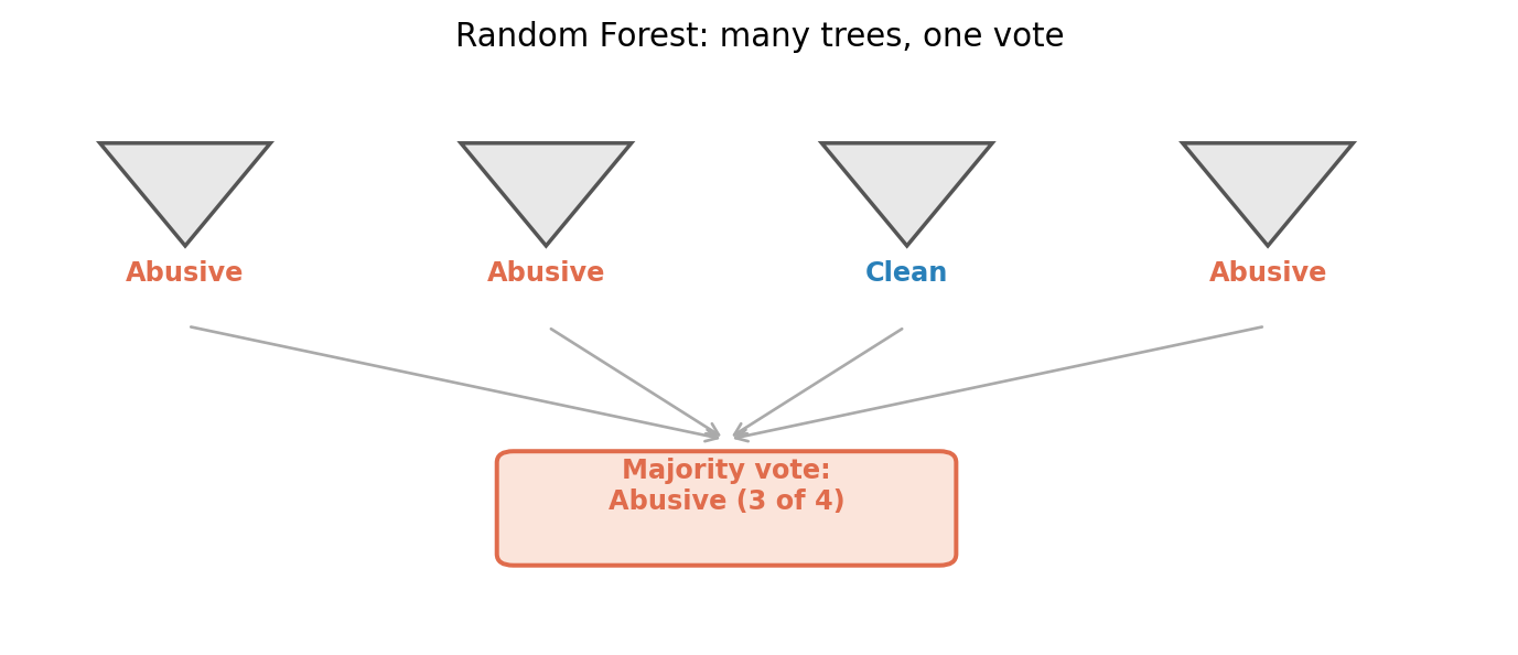
• To classify a new message, every tree votes — the majority wins

Random Forest, Visualized

Any single tree can overfit. A crowd of imperfect trees, voting together, usually can’t.

Wrap-Up

What We Built This Week

• Tokenization — turning raw chat messages into words
• Count vectors — turning words into numbers
• Naive Bayes — a probabilistic classifier, built from those numbers
• Bigrams / n-grams — recovering a little bit of word order
• TF-IDF — weighting words by how distinctive they are
• Decision trees / forests — a rule-based alternative, no independence assumption

Back to Where We Started

viewer1: trash uninstall noob

viewer2: well played gg

viewer3: you're actually trash at this game

viewer4: that boss fight will kill me 😭

• We now have several ways to answer “is this abusive?” — probabilistically, or rule-by-rule
• But message 4 is exactly the kind of case that still trips these models up: “kill” in a game complaint, not a threat
• No model here truly understands the message — each is finding statistical patterns in word usage

One Thing Worth Sitting With

• These models learn whatever patterns exist in their training data — including its blind spots
• Abuse classifiers built this way have been shown to flag African American English and reclaimed language as abusive at disproportionately higher rates, simply because of the word patterns involved
• A “highly accurate” classifier can still be systematically wrong for specific groups of people

As designers of these systems, the question isn’t just “does this model work?” — it’s “who does it work for, and who does it fail?”